 |
KSFoundation
[May-2021]
A platform for simpler EPIC programming on GE MR systems
|


|
|
KSFoundation
[May-2021]
A platform for simpler EPIC programming on GE MR systems
|
|
Home
There are two types of plot modes for sequence drawing in the KSFoundation library: HOST (ks_plot_host()) and TGT/IPG (ks_plot_tgt_addframe()).
In addition, there is a slice-timing graph that is generated on HOST via ks_plot_slicetime().
/usr/local/anaconda2/usr/local/bin/apython -> /usr/local/anaconda2/bin/python plot subdirectory of the current psd folder/usr/g/mrraw/plot/<psdname>
Plotting your sequence on HOST allows you to visualize the sequence after the pulsegen function(s) have been dry-runned on HOST, before any waveforms have been created on TGT. The benefit with this is that one can look for e.g. gradients that may overlap before the related hardware (TGT) error occurs. Please note that a call to the sequence's seqstate function should be done to set the amplitudes of the phase encoding gradients for a given shot:
Note that the acquisition windows are presented together with the frequency encoding gradient, and will also show up differently if ramp sampling is applied.
Plotting in HOST mode is supported on both Sim (WTools) and on the MR scanner. Plotting in TGT mode is supported on Sim only to avoid end-of-sequence (EOS) interrupts while scanning.
In addition, there is a slice-time plotting feature using ks_plot_slicetime() (see Slice-time plotting of multiple sequence modules below).
All plot calls below are already set up for the provided psds, please see:
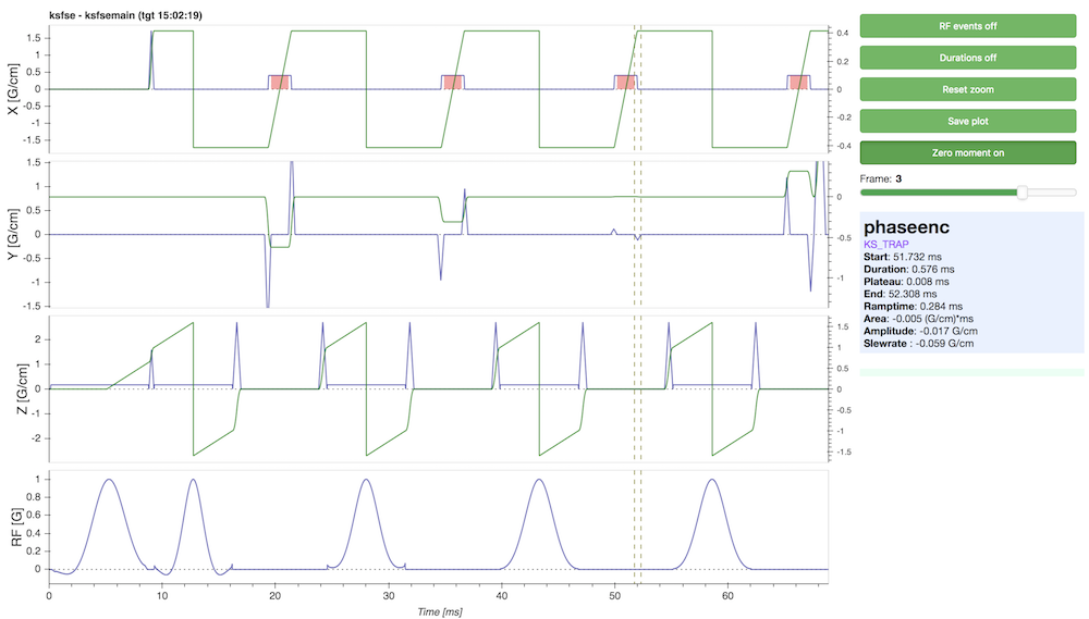
The benefit of plotting on TGT is to see scan time changes such as phase encoding variations. Depending on what you want to visualize, place the call to ks_plot_tgt_addframe(...) in the corresponding scan function.
predownloadctrl is the sequence module you want to plotopslquant = 1 may help.if you want to visualize the phase encoding steps in the ksfse sequence:
ks_plot_tgt_addframe() in ksfse_scan_acqloop(): You can change the fileformat (default PNG) with the CV ks_plot_filefmt.
Helvetica font is the default font but is not required.
Check psdplot.py for further customization.
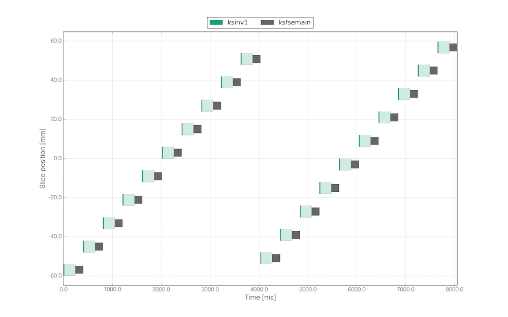
Adding a ks_plot_slicetime() command right after every ks_scan_playsequence() call in the sequence (main sequence + optional additional sequence modules) provides the information necessary to automatically create a slice-time plot for the sequence with time on the X-axis and slice location on the Y-axis. In this slice-time plot, each sequence module is plotted as a box, where the box height corresponds to the slice thickness of the current sequence module and the box width corresponds to the duration of the sequence module (<module>.seqctrl.duration). If .seqctrl.duration is larger than .seqctrl.min_duration for a sequence module, the time after .seqctrl.min_duration up to .seqctrl.duration will be shown in pale color (as for ksinv1 in the figure above). This indicates that the sequence module has some dead time after the last waveforms in the sequence module.
Note that this plot is generated on HOST in predownload() and works both for SIM and HW.
For SIM (WTools), the slice-time plot will be placed in ./plot/slicetime/<psdname>_slicetime.png. For HW (MR-scanner), the plot will be generated when SaveRx is pressed and placed in /usr/g/mrraw/plot/<psdname>/slicetime/<psdname>_slicetime.png.
ks_plot_slicetime() can take multiple slice locations (in [mm]) as arguments to be able to plot SMS (multi-band) sequence data.
See also ks_plot_slicetime_begin() and ks_plot_slicetime_end()
In ksgre.e, ksfse.e and ksepi.e, and the provided sequence modules, ks_plot_slicetime() is already added after each call to ks_scan_playsequence().
Here is an example for ksfse with inversion:
From the main sequence (ksfse_implementation.e):
From the @include'd inversion code (KSInversion.e), a bit simplified without SMS:
See also how the following calls are placed in ksfse_scan_acqloop() to mark end of slice-groups & passes for the slice timing plot:
From ksfse_predownload_plot():
 1.8.14